So far in this series, we’ve dealt with the qualitative detection of molecular targets—that is, a basic assessment of whether the target is present or absent within a test sample. In many cases, still further information of clinical utility can be achieved by obtaining quantitative information: that is, a measure of how much of a specific molecular target is present. Some prime examples of where this sort of information can be used include:
- Monitoring of viral load in solid organ transplant recipients. The use of immunosuppressive agents in this context to stop transplant rejection can allow the reactivation of long dormant prior infections (EBV or CMV are particularly well known examples) with very serious consequences. Regular monitoring of patients can allow adjustments in immunosuppressive therapy to achieve a balance between transplant rejection and viral reactivation.
- Gene expression information. Quantitative reverse-transcription PCR (qRT-PCR) can be employed to measure and quantify even very small amounts of transcription and assess expression regulation in response to environmental stimuli.
- Detection of copy number variations (CNVs), in the form of very small deletions or duplications of chromosomal regions.
- Differentiation of an ongoing pathogen infection from residual positivity arising from a prior infection or an inactive viral integrant. (A particularly fascinating example of this is in the context of suspected HHV-6 infection. A sizeable proportion of the population carries inactive HHV-6 integrants, resulting in clear, strong positive HHV-6 PCR results on samples such as peripheral whole blood due to the white cell content. A quantitative result showing HHV-6 loads well above WBC count levels for a sample is therefore beneficial in helping distinguish true infections. In this particular case other clinical assessment and test strategies can also be employed, but they’re beyond the scope of the topic of this chapter of “The Primer.”)
Of course, other non-PCR methods exist for gathering similar data. Serological methods, expression arrays (molecular in nature but not PCR based), and array comparative genome hybridization (array CGH, again molecular but non-PCR based), for instance, could be applied in the above examples as methods for extracting similar information. The advantages of quantitative PCR (qPCR) or its RNA cousin, qRT-PCR, arise from the by now familiar points of rapid test performance, high sensitivity, excellent specificity, and ease of adaptation to new targets which are inherent in molecular amplification based approaches.
It didn’t take long after the development of classical PCR for people to appreciate the potential power of somehow extracting quantitative data from the method. A serious technical hurdle, however, was that the PCR method is inherently not well suited for quantitation. The reasons for this are simple. By their nature, successful PCR reactions exponentially use up resources such as primers or dNTPs present in the reaction tube. As these resources become depleted, the reaction slows and eventually stops. In a sample where a large amount of target template was present, this process occurs early; where less target template was present, it occurs later (Figure 1). As a rule of thumb, in a well designed PCR reaction nearing theoretical maximum 2N efficiency, a reaction starting from a single target copy will essentially plateau when around 1012 amplicons have been made. This corresponds to about 40 thermocycles in a perfect reaction (240 = 1.1×10¹², for those of you wishing to follow the math). This in turn relates to why 40 is a commonly used maximum number of cycles in PCR and RT-PCR methods. (Adding more cycles won’t tend to help truly positive reactions go further, and allows greater chances of spurious side reactions leading to false positive signals. Conversely, if a PCR protocol requires much more than 40 cycles, it’s a good indication it’s poorly optimized).
Figure 1. Amplification curves from a real-time PCR on 10-fold serial dilutions of a positive target—from 2.5e8 GEq/ml (leftmost) to 2.5e4 Geq/ml (rightmost). Locations of threshold, and plateau level are indicated. Individual reactions curves crossing threshold (CT or CP) are indicated with arrows.
The result of this is that one can’t just run a PCR, run the product on a gel (or hybridize it to an array, or any other direct endpoint detection method), and accurately judge the starting template copy number from the signal intensity. This is in effect measuring the endpoint signal level, and as we can see in Figure 1, all the reactions end up at the same place: the “plateau phase.” At the very far extremes of template load—from very high to barely there at all—there can sometimes be a small difference seen, but across many logs of “mid-range” concentrations, no reliable correlation is observed. In fact, differences in plateau can arise from factors unrelated to template concentration, leading to wildly erroneous results if the final amplicon level is assumed to relate to starting template load.Early on, two methods were devised to try to get around this problem. The first was to make an artificial “competitor” template, sharing the same PCR primers as the target, but with an internal “stuffer” sequence resulting in a differently sized product, resolvable from the real target on an agarose gel. By titrating in a range of known quantities of this competitor template to a sample, running regular PCR and gel analysis, and observing the point at which the competitor-derived band approximates the intensity of the intrinsic target in a sample, one can make an estimate of the target load as being similar to the competitor load. While potentially skewed by effects such as non-identical amplification efficiencies of the two competing targets, the method is technically simple and reasonably effective. It has, however, been almost completely supplanted by newer, much more accurate and less tedious methods described below.
The second early method was similarly simple, and conceptually similar to the Reed-Muench approach readers may be familiar with for calculating titres. Here, one prepares a range of serial dilutions of a sample, and performs multiple replicate PCRs on each dilution point, with some endpoint qualitative detection method such as agarose gel to score the reactions as positive or negative. For any starting template concentration, there is obviously some point at which serial dilution can effectively remove any templates from most of the samples taken from that dilution. Statistical analysis of large numbers of reactions across the dilution range where the assays start to show a mixture of positive and negative results can be employed to calculate the initial sample target concentration. While theoretically robust, the method was cumbersome and tedious in the extreme, as the author can personally attest. Recently however this method has had something of a resurgence in the form of “digital drop PCR” and similar methods whereby automation and microfluidics can do all of the dilutions, very many of the PCR reactions, assessment of individual micro-reaction positivity or negativity, and mathematical analysis, followed by generation of a numerical result. A strength of this approach is that it is intrinsically an absolute quantitation; that is, it does not have to refer to an external standard curve for interpretation. Automation has thus given new life to this approach, and this approach is becoming more widespread. Look for it to arrive soon in a lab near you.
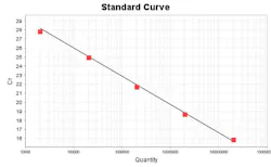
The most common methods of qPCR in use today all, however, hinge around real-time approaches. Again going back to Figure 1, the reader will notice that there very clearly is one aspect of the reaction signals which correlates with starting template copy number: the number of PCR cycles required before a signal rises up out of the fluorescence noise floor to cross a “threshold” value (indicated by arrows in Figure 1). This point in an amplification curve, expressed in cycle number, is referred to as the “cycle crossing threshold” (CT) or “crossing point” (CP) on differing systems but with the same import. The more starting target template, the earlier this occurs. While perhaps not surprising, what is particularly nice about this observation is that when log (starting template) is plotted against CT (or CP if you prefer), the result is beautifully linear, often across six logs or more, in starting template concentration. As an example, see Figure 2, which is this form of plot based on the same amplification plot data shown in Figure 1.
Figure 2. Standard curve generated from the data in Figure 1. (NOTE: Threshold applied by instrument software is not precisely that shown for example in Figure 1. CT values differ slightly as a result).
Application of this approach requires one to generate a standard curve for your reaction, using some form of quantified target with a known value for your template to create a serial dilution and prepare a standard curve for reference. As such, this is, strictly speaking, a form of relative quantitation, as you assess your test sample CT (CP) against a standard and the accuracy of your results hinges on the accuracy of the standard curve. Regardless, the simplicity and wide dynamic range of this method have made it the most common approach for qPCR and qRT-PCR applications today.
When considering this method, some things to note: First, the method of selecting CT / CP can have some influence in the quality of the standard curve. Different algorithms are used by different real-time PCR instrument systems, and allow varying degrees of user control over the algorithm (boxcar averaging, mode of background subtraction, manual setting against amplification curves, etc.). Thus, unless some sort of shared reference is compared between assays and systems, direct comparison of absolute quantity values returned by different systems isn’t very meaningful. Note however that relative quantities between samples, as reported on different systems, are still generally similar (that is, a five-fold difference between samples will look like a five-fold difference regardless).
This approach is amenable to both binding dye (such as SYBR green) based real-time PCR and probe-based methods covered in previous installments of this series. Where applied to binding dye-based results, bear in mind that the amplification curves obtained and used for measuring quantity may contain contributions from side reactions such as primer dimers. Assessment of melt curves is useful here, with reactions showing only one significant product peak being the most accurately assessed by CT/CP. In the case where small amounts of artefact products are seen along with the expected product peak, some compensation can be attempted by using relative peak areas within the melt curve to assess what proportion of amplification curve signal arises from the correct product, but accuracy is compromised. Due to their more specific signal nature, probe-based real time PCR or RT-PCR approaches are preferable for qPCR (and qRT-PCR) applications where practical.
Regardless of format, qPCR approaches can give the clinician valuable data not otherwise available, and more and more assays are beginning to be provided in this format.
About the Author

John Brunstein, PhD
is a member of the MLO Editorial Advisory Board. He serves as President and Chief Science Officer for British Columbia-based PathoID, Inc., which provides consulting for development and validation of molecular assays.


