Limits of detection—is not detected always synonymous with not present?
Let’s start this month’s episode with a quick reminder of the target audience for this series—that is, the non-specialist interacting with molecular testing methods. If you’re an expert in MDx none of the following is going to be news to you. However, judging by questions I repeatedly encounter, for your colleagues who don’t specialize in the arcane depths of clinical nucleic acid testing, the following may clarify what some of the underlying caveats are any time a molecular assay returns a negative result. With this in mind, let’s consider a situation where a reliable, properly validated, and properly performed molecular test such as a PCR for the presence of a particular infectious organism, yields a negative result. What does that actually mean?
Poisson is not your friend (unless you’re running digital PCR)
Well, here’s a name that keeps popping up over the life of this series—Siméon Denis Poisson, French mathematician. Among other things, he examined the statistics around sampling. If you have a number of discrete items randomly distributed within a container, and you have a way of counting these items and count the whole container, you will get an accurate measurement of the number of items. If however you take a sub-portion sample of the container and count items in that, you may not get an accurate count. If your container has one countable item and your sample is 1/10 of the container, your most likely result would be not counting the item (your conclusion—container doesn’t have any of the item, which is clearly wrong). Of course, your other possible result—that you got lucky and your sample happened to capture the one item—is also misleading from a quantitative standpoint, as you’d assume the whole sample likely has ~10 items. These sorts of misleading results occur when the target analyte is at low real numbers (low concentrations) and become increasingly less of an issue either theoretically or practically, as numbers increase such that the sample is more likely to have a representative number of items. Note that this could be due to increasing analyte concentration, or to increasing sample size; we’ll come back to this later.
What does this mean from a practical standpoint? Well, it turns out this has been considered in depth in various validation strategies and guidance documents. You may have run across types of assays which include what are called both a “low positive” and a “high positive” control. By the usually accepted definition, a low positive control is one which gives a positive assay result 19 times out of 20 (95 percent). That’s right, you read that correctly. We call it a positive control and if everything is working perfectly, about 5 percent of the time it should be negative. In fact, if you’re not seeing that, you’re doing something wrong and probably getting excessive false positives! (Note, however, if you have such an assay with a formal “low positive,” this doesn’t mean you should be overly worried if you run 20 consecutive tests on it and don’t get a negative. If, however you can go to 3x the 5 percent frequency level—that is, if you can do 60 sequential tests and still not get a single negative, Poisson says in a nutshell that you’ve likely got a problem. Over very large numbers of tests you should see 5 percent negative rate for this type of control but for any given series of 20 it would not be unusual to see either no negatives, or perhaps two negatives. Neither is cause for alarm.)
If you have true positive samples at analyte concentrations near that of a low positive, the simple fact is that you’re going to report false negatives roughly 5 percent of the time.
Take cheer though that Poisson wasn’t all bad news for MDx; if you want to know how his work underpins the magic of digital PCR and allows us to quantitate targets without need for standard curves, have a look back at this space from the December 2013 issue.
A little inhibition goes a long way
Our next culprit in obscuring whether a test negative is a true negative is assay inhibition. “Nonsense!” is the response. “I have an internal control which warns me of this!” Well, actually, the interpretation is a little more complicated than that. While qualitative and quantitative internal controls (IC) work a bit differently and we’ll consider each case in turn, failure of IC in either context leaves you with a non-meaningful result. It will stop you from calling a false negative, true, but you’re left unable to say whether the sample in question is either positive or negative.
Internal controls are least informative in qualitative assay context. We don’t want the IC signal to be sporadically failing for no reason, so it’s generally at a level several times (at least 3-4x) that of a formal low positive (assuming equal detection efficiencies between IC and real analyte). Thus, when IC fails, we can be sure there’s at least enough assay inhibition going on to supress detection of true targets at 3-4x a low positive level. If there’s just slightly less inhibition though, we get into a zone where the qualitative IC can still be positive but the actual functional limit of detection (LOD) is no longer what we expect it to be. Of course if the IC levels are even higher, then this zone of partial inhibition where true analytes can drop out while we are blithely unaware, becomes even larger.
Quantitative contexts such as real-time PCR are a bit clearer, if we assume that the degree of inhibition observed for the IC is the same as that for target analyte. Unless we have evidence to the contrary, that seems reasonable enough. A 1 CT (or CP, crossing threshold or crossing point depending on your platform and terminology of preference) increase in IC corresponds to a 2-fold loss in sensitivity; put another way, your analyte LOD has just gone up by a factor of two, say from 200 U/ml to 400 U/ml. Usually with a qualitative IC, there will be some accepted rules or guidelines as to what sort of a shift in IC CT (CP) is allowed before all analyte results are called into question or discarded as not reportable.
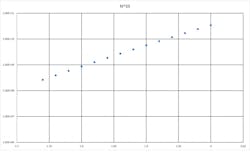
For the mathematically inclined, it’s interesting to consider how a drop in per-cycle PCR efficiency relates to loss of overall sensitivity. Recall that an ideal PCR is a doubling (x2) per cycle, the theoretical yield of PCR product for N thermocycles is 2^N. Inhibition acts to reduce 2 to a smaller number, say 1.8. That’s only a 10 percent loss in efficiency, but the exponential nature of the process amplifies that error. Using some hard numbers, say 35 cycles, a perfect PCR would yield 2.44e10 products, while the 10 percent inhibited assay only yields 1.27e9 products—or about a 19 fold loss. If this were our above example with an ideal LOD of 200 U/ml, it’s now 3843 U/ml.
In either context, the bottom line is that there’s potential for there to be some degradation of assay performance before it’s going to fully supress internal control signals, and this is a window of opportunity for false negative results.
Legend. Theoretical amplicon yields at 35 cycles vs per-cycle PCR efficiency, at 35 cycles.
Reaction volumes—size matters
There was a promise above that we’d return to the issue of sample size. In this context we mean “amount of template/extract volume put in the reaction,” as opposed to the size of the original specimen. I was recently approached by the sales representative for an unnamed company, who proceeded to wax lyrical about their new PCR platform with 1.2 μl reaction volumes; not nearly as tiny as digital PCR range, but certainly smaller than reactions volumes on most common platforms. If we take that to be around 25 μl—make it 24 μl for simplicity—it’s 20 times smaller.
Of course, there are some real advantages to this. Per reaction reagents cost is lowered, and thermal mass is smaller, meaning shorter dwell times needed in thermo-cycling, and concurrent faster whole reaction times. However, all other things being equal—including ratio of template to PCR reagents per reaction—then using this platform one can only put 1/20 as much extract in the reaction as you could in a 24 μl reaction and simplistically, we’ve just raised our LOD by 20x as compared to running the larger volume reaction. In the early days of real-time PCR, there were even such things as 100 μl reactions which would allow for sampling ~80x more input material per reaction.
This particular line of logic is mostly pertinent to the LOD value observed in the assay validation, and where the balance between reagent cost savings and required LOD lies. For what are expected to be high copy number analytes, small reaction volumes can be great—but applying them if low range sensitivity is required may be counterproductive. Like most fields, different tools are better suited for different jobs.
Sequence variation
Finally, what about target genetic variability? MDx assay developers go to great lengths to try to find ideal, well conserved/consensus primer binding sites. These help ensure that biological pressure on the target analyte/organism limits variation off from these sequences but it’s not an absolute guarantee. Especially if the analyte is an emerging organism, one for which there are necessarily limited example sequences to base primer design on, it’s within the realm of possibility that you could encounter an organism with critical sequence variations under primer and/or probe binding sites. Depending on where and what these nucleotide changes are, they may cause very significant losses in assay sensitivity and lead to false negative results.
Absence of proof is not proof of absence—traditional aphorism
Fortunately, the single most likely reason for a well designed, well validated, and properly run MDx assay to return a negative result is that the sample doesn’t contain the analyte in question. All of the above however should serve to remind the end user of any assay that while rare, false negatives can and do occur. In the MDx context we considered there are a number of factors which can contribute to this. All of this goes to underline the importance of interpreting lab results in real context and being ready to question them if they really don’t seem to fit. In such cases retesting or use of an alternate secondary assay may be wise.
About the Author

John Brunstein, PhD
is a member of the MLO Editorial Advisory Board. He serves as President and Chief Science Officer for British Columbia-based PathoID, Inc., which provides consulting for development and validation of molecular assays.

